Sums of Kronecker terms

In some instances a single Kronecker term will not be enough to model a physical system. A star, for instance, may exhibit variability on timescales of days due to rotational modulation and variability and on timescales of minutes to hours due to surface convection. If these two different sources of variability shift the star’s spectrum in different ways then the amplitude of the variability will differ with timescale. Modeling this situation will therefore require us to use two Kronecker terms, one to model the wavelength-dependence of the rotationally modulated variability and the other for the convection driven variability.

In this tutorial we will construct two different GP models out of sums of Kronecker-structured covariance matrices. In another tutorial we’ll use a similar sum to fit solar variability.

To start, we’ll define two celerite terms with different characteristic frequencies.

import numpy as np
import exoplanet as xo

term1 = xo.gp.terms.SHOTerm(log_S0=-3.0, log_w0=2.0, log_Q=-np.log(np.sqrt(2)))
term2 = xo.gp.terms.SHOTerm(log_S0=5.0, log_w0=-1.0, log_Q=-np.log(np.sqrt(2)))

We can combine these with two different scaling vectors using specgp and define a GP from the resulting kernel:

import specgp as sgp

kronterm1 = sgp.terms.KronTerm(term1, alpha=[1, 3, 5])
kronterm2 = sgp.terms.KronTerm(term2, alpha=[5, 3, 1])

kernel = kronterm1 + kronterm2

t = np.linspace(0, 10, 1000)
gp = xo.gp.GP(x=t, kernel=kernel, diag=0.001 * np.ones((3, len(t))), mean=sgp.means.KronMean(np.zeros((2, len(t)))), J=4)

Now let’s take a look at a random realization of the GP:

import matplotlib.pyplot as pl
%matplotlib inline

n = np.random.randn(3*len(t), 1)
y = gp.dot_l(n).eval()

pl.plot(t, y[::3], color='#FE4365', linewidth=3)
pl.plot(t, y[1::3], color='#3F9778', linewidth=3)
pl.plot(t, y[2::3], color='#00A9FF', linewidth=3)
pl.ylabel('y')
pl.xlabel('time')

Text(0.5, 0, 'time')

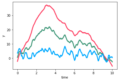
We can clearly see two different timescales of variability and that they have different wavelength-dependencies. On long timescales the amplitude of the variability increase as we go from the blue to the green to the red curve, but on short timescales the opposite is true: the amplitude of the short timescale variability decreases from blue to red. This behavior cannot be captured by a single KronTerm.

Another case in which one may want to combine multiple Kronecker terms is the case in which two processes share a common source of variability but also have their own independent variabilities. For instance, two stars that are observed at the same time via the same instrument will have the same systematics, but with their own variability superimposed. Let’s see how we can reproduct this situation using a sum of KronTerms. We begin by defining celerite terms for the common variability and each of the independent processes:

common_term = xo.gp.terms.SHOTerm(log_S0=10.0, log_w0=-2.0, log_Q=-np.log(np.sqrt(2)))
ind_term1 = xo.gp.terms.SHOTerm(log_S0=-2.0, log_w0=2.0, log_Q=-np.log(np.sqrt(2)))
ind_term2 = xo.gp.terms.SHOTerm(log_S0=-2.0, log_w0=2.0, log_Q=-np.log(np.sqrt(2)))

If we want the common term to have the same amplitude at each wavelength, then the scaling vector should be [1, 1]. For the independent terms, the scaling vectors will be [1, 0] and [0, 1] so that the amplitude of the unwanted term is zero’d out for each time series:

common_alpha = [1, 1]
ind_alpha1 = [1, 0]
ind_alpha2 = [0, 1]

kernel = (sgp.terms.KronTerm(common_term, alpha=common_alpha) +
          sgp.terms.KronTerm(ind_term1, alpha=ind_alpha1) +
          sgp.terms.KronTerm(ind_term2, alpha=ind_alpha2))

We define a GP with this kernel, this time setting J=6 (J increases by 2 for each SHOTerm).

gp = xo.gp.GP(x=t,
              kernel=kernel,
              diag=0.001 * np.ones((2, len(t))),
              mean=sgp.means.KronMean(np.zeros((2, len(t)))),
              J=6)

As before we can visualize the GP is by examining a random realization:

n = np.random.randn(2*len(t), 1)
y = gp.dot_l(n).eval()

pl.plot(t, y[::2], color='#FE4365', linewidth=3)
pl.plot(t, y[1::2], color='#3F9778', linewidth=3)
pl.ylabel('y')
pl.xlabel('time')

Text(0.5, 0, 'time')

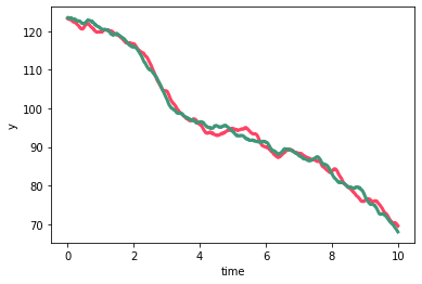
And, as constructed, we see that the two timeseries share the long-timescale, large-amplitude variability while the shorter timescale lower amplitude variability is unique to each timeseries.