Getting started

This tutorial covers the basics of computing 2D GPs with exoplanet using the classes provided by specgp. For a more complete tutorial on using celerite in exoplanet, check out the exoplanet docs. If you’re not familiar with exoplanet, it might be helpful to take a look at some of those tutorials before working through these.

exoplanet and specgp are primarily intended for use with pymc3. For this reason all variables used by specgp are stored as nodes in a computational graph in the form of theano tensors. This means that in order to compute the actual value of a variable outside of the pymc3 model context, we’ll need to periodically call .eval() to get the actual values of these nodes.

To start, let’s define a 1D celerite term:

import numpy as np
import exoplanet as xo

term = xo.gp.terms.SHOTerm(log_S0=0.0, log_w0=1.0, log_Q=-np.log(np.sqrt(2)))

Here we’ve chosen the simple harmonic oscillator (SHO) term, which is a commonly used model for stellar variability. The choice is somewhat arbitrary; specgp works with any celerite term.

If we’re only working in one dimension we can define the GP with this kernel alone. Here diag is the white noise variance for the GP and J is the width of the system (each SHOTerm contributes J=2 to the total width).

t = np.linspace(0, 10, 1000)
gp = xo.gp.GP(
                x=t,
                kernel=term,
                diag=0.01 * np.ones_like(t),
                mean=xo.gp.means.Constant(0.0),
                J=2
              )

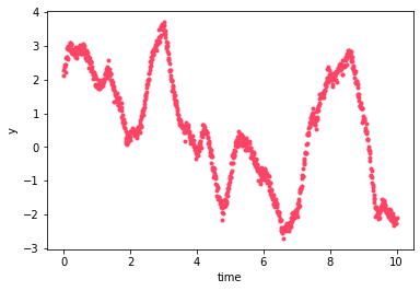
Let’s take a look at a random realization of this GP:

import matplotlib.pyplot as pl
%matplotlib inline

n = np.random.randn(len(t), 1)
y = gp.dot_l(n).eval()

pl.plot(t, y, '.', color='#FE4365')
pl.xlabel("time")
pl.ylabel("y")

Text(0, 0.5, 'y')

What if we want to model two timeseries that have the same underlaying variability? This is where specgp comes in. It provides a class, KronTerm that defines a Kronecker-structured covariance matrix for computing a 2D GP (which can also be thought of as a collection of correlated 1D GPs).

import specgp as sgp

# scaling factor for each process
alpha = [1, 2]
kernel = sgp.terms.KronTerm(term, alpha=alpha)

For the 2D GP, both diag (the white noise variances for each input coordinate) and mean (the value of the GP mean for each input coordinate) are two dimensional:

# the white noise components for each process
# here we set the second process to have 100 times the white noise
# variance of the first.
diag = np.array([0.001, 0.1])
diag = diag[:, None] * np.ones_like(t)
print(diag)

[[0.001 0.001 0.001 ... 0.001 0.001 0.001]
 [0.1   0.1   0.1   ... 0.1   0.1   0.1  ]]

For the the GP mean we need to use the provided KronMean mean function which is compatible with the KronTerm kernel. KronMean defines a constant mean function. We give it two values, each being the (constant) mean of one of the processes:

mu = sgp.means.KronMean(np.zeros((2, len(t))))

Finally, we can define the 2D GP:

gp = xo.gp.GP(x=t, kernel=kernel, diag=diag, mean=mu, J=2)

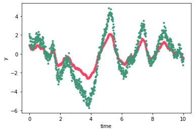
Let’s take a look at a realization of this GP:

n = np.random.randn(2*len(t), 1)
y = gp.dot_l(n).eval()

pl.plot(t, y[::2], '.', color='#FE4365')
pl.plot(t, y[1::2], '.', color='#3F9778')
pl.xlabel("time")
pl.ylabel("y")

Text(0, 0.5, 'y')

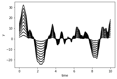
A quick note on the structure of the vector returned by dot_l: y is a 1D vector with the first 2 elements consisting of the first observation for each of the two processes, the next two being the second observation at each wavelength, and so forth. We could also write \(y = vec(Y)\) where \(Y\) is a matrix of size \(2\times N\) with \(N\) the number of times and with each of the rows containing the timeseries of one of the correlated processes. For \(M\) correlated processes the first \(M\) elements of \(y\) are the observation at the first time for each process, and so forth:

nprocesses = 10

alpha = np.linspace(1, 10, nprocesses)
kernel = sgp.terms.KronTerm(term, alpha=alpha)

diag = np.array([0.01] * nprocesses)
diag = diag[:, None] * np.ones_like(t)

mu = sgp.means.KronMean(np.zeros((2, len(t))))
gp = xo.gp.GP(x=t, kernel=kernel, diag=diag, mean=mu, J=2)

n = np.random.randn(nprocesses*len(t), 1)
y = gp.dot_l(n).eval()

for i in range(nprocesses):
    pl.plot(t, y[i::nprocesses], '-', color='k')
pl.xlabel("time")
pl.ylabel("y")

Text(0, 0.5, 'y')